Lesson 3. Model Tuning

Notebook supporting the video series "Using MLJ".

Slides from the video.

To run the code in this tutorial in a live Julia session, first follow the instructions given here.

Part I. Learning Curves

using MLJ, Plots
RandomForestRegressor = @load RandomForestRegressor pkg=DecisionTree

X, price = @load_reduced_ames;
schema(X)

┌──────────────┬───────────────────┬──────────────────────────────────┐
│ names        │ scitypes          │ types                            │
├──────────────┼───────────────────┼──────────────────────────────────┤
│ OverallQual  │ OrderedFactor{10} │ CategoricalValue{Int64, UInt32}  │
│ GrLivArea    │ Continuous        │ Float64                          │
│ Neighborhood │ Multiclass{25}    │ CategoricalValue{String, UInt32} │
│ x1stFlrSF    │ Continuous        │ Float64                          │
│ TotalBsmtSF  │ Continuous        │ Float64                          │
│ BsmtFinSF1   │ Continuous        │ Float64                          │
│ LotArea      │ Continuous        │ Float64                          │
│ GarageCars   │ Count             │ Int64                            │
│ MSSubClass   │ Multiclass{15}    │ CategoricalValue{String, UInt32} │
│ GarageArea   │ Continuous        │ Float64                          │
│ YearRemodAdd │ Count             │ Int64                            │
│ YearBuilt    │ Count             │ Int64                            │
└──────────────┴───────────────────┴──────────────────────────────────┘

y = price/100_000; # price in multiples of $100,000
first(y, 5)

5-element Vector{Float64}:
 1.38
 3.699
 1.8
 2.075
 1.47

Define a model and a "dummy" model for baseline comparison:

model = RandomForestRegressor(
    rng=123,
    n_subfeatures=1,
)
pipe =  ContinuousEncoder() |> model
baseline = ContinuousEncoder() |>  ConstantRegressor();

Get a performance baseline:

options = (; resampling=CV(nfolds=3), measure = mae, acceleration=CPUThreads())
e0 = evaluate(pipe, X, y; options...)
ebase = evaluate(baseline, X, y; options...)

PerformanceEvaluation object with these fields:
  model, tag, measure, operation,
  measurement, uncertainty_radius_95, per_fold, per_observation,
  fitted_params_per_fold, report_per_fold,
  train_test_rows, resampling, repeats
Tag: ProbabilisticPipeline-112
Extract:
┌──────────┬──────────────┬─────────────┐
│ measure  │ operation    │ measurement │
├──────────┼──────────────┼─────────────┤
│ LPLoss(  │ predict_mean │ 0.568       │
│   p = 1) │              │             │
└──────────┴──────────────┴─────────────┘
┌──────────────────────┬─────────┐
│ per_fold             │ 1.96*SE │
├──────────────────────┼─────────┤
│ [0.544, 0.57, 0.592] │ 0.0332  │
└──────────────────────┴─────────┘

Inspect hyper-parameters:

pipe

DeterministicPipeline(
  continuous_encoder = ContinuousEncoder(
        drop_last = false, 
        one_hot_ordered_factors = false), 
  random_forest_regressor = RandomForestRegressor(
        max_depth = -1, 
        min_samples_leaf = 1, 
        min_samples_split = 2, 
        min_purity_increase = 0.0, 
        n_subfeatures = 1, 
        n_trees = 100, 
        sampling_fraction = 0.7, 
        feature_importance = :impurity, 
        rng = 123), 
  cache = true)

Define a 1D hyper-parameter range:

r = range(pipe, :(random_forest_regressor.n_trees), lower=10, upper=500)

NumericRange(10 ≤ random_forest_regressor.n_trees ≤ 500; origin=255.0, unit=245.0)

A learning_curve has the same arguments as evaluate except but with extra range option:

curve = learning_curve(
    pipe, X, y;
    range=r,
    resampling=Holdout(fraction_train=0.8),
    measure=mae,
)
plt = plot(curve.parameter_values, curve.measurements)
savefig("learning_curve.svg");

[ Info: Training machine(DeterministicTunedModel(model = DeterministicPipeline(continuous_encoder = ContinuousEncoder(drop_last = false, …), …), …), …).
[ Info: Attempting to evaluate 30 models.
Evaluating over 30 metamodels:   7%[=>                       ]  ETA: 0:00:01[KEvaluating over 30 metamodels:  10%[==>                      ]  ETA: 0:00:01[KEvaluating over 30 metamodels:  13%[===>                     ]  ETA: 0:00:01[KEvaluating over 30 metamodels:  17%[====>                    ]  ETA: 0:00:01[KEvaluating over 30 metamodels:  20%[=====>                   ]  ETA: 0:00:01[KEvaluating over 30 metamodels:  23%[=====>                   ]  ETA: 0:00:02[KEvaluating over 30 metamodels:  27%[======>                  ]  ETA: 0:00:02[KEvaluating over 30 metamodels:  30%[=======>                 ]  ETA: 0:00:02[KEvaluating over 30 metamodels:  33%[========>                ]  ETA: 0:00:03[KEvaluating over 30 metamodels:  37%[=========>               ]  ETA: 0:00:03[KEvaluating over 30 metamodels:  40%[==========>              ]  ETA: 0:00:03[KEvaluating over 30 metamodels:  43%[==========>              ]  ETA: 0:00:04[KEvaluating over 30 metamodels:  47%[===========>             ]  ETA: 0:00:04[KEvaluating over 30 metamodels:  50%[============>            ]  ETA: 0:00:04[KEvaluating over 30 metamodels:  53%[=============>           ]  ETA: 0:00:05[KEvaluating over 30 metamodels:  57%[==============>          ]  ETA: 0:00:05[KEvaluating over 30 metamodels:  60%[===============>         ]  ETA: 0:00:05[KEvaluating over 30 metamodels:  63%[===============>         ]  ETA: 0:00:05[KEvaluating over 30 metamodels:  67%[================>        ]  ETA: 0:00:05[KEvaluating over 30 metamodels:  70%[=================>       ]  ETA: 0:00:05[KEvaluating over 30 metamodels:  73%[==================>      ]  ETA: 0:00:05[KEvaluating over 30 metamodels:  77%[===================>     ]  ETA: 0:00:05[KEvaluating over 30 metamodels:  80%[====================>    ]  ETA: 0:00:05[KEvaluating over 30 metamodels:  83%[====================>    ]  ETA: 0:00:04[KEvaluating over 30 metamodels:  87%[=====================>   ]  ETA: 0:00:04[KEvaluating over 30 metamodels:  90%[======================>  ]  ETA: 0:00:03[KEvaluating over 30 metamodels:  93%[=======================> ]  ETA: 0:00:02[KEvaluating over 30 metamodels:  97%[========================>]  ETA: 0:00:01[KEvaluating over 30 metamodels: 100%[=========================] Time: 0:00:36[K

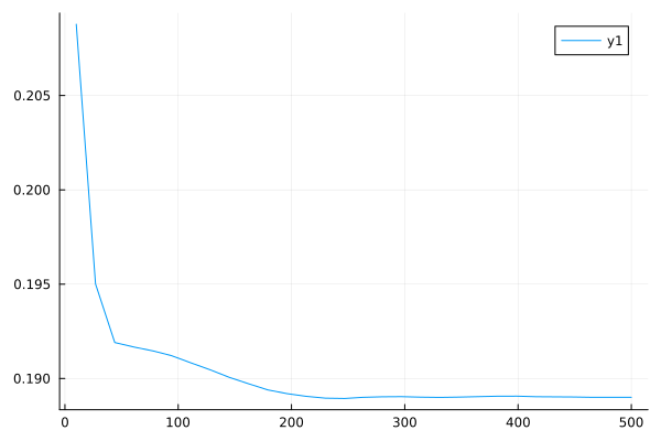
Let's set n_trees to a a value that looks sufficient to get convergence:

pipe.random_forest_regressor.n_trees = 250;

Part II. The `TunedModel` Wrapper

r1 = range(pipe, :(random_forest_regressor.n_subfeatures), lower=1, upper=12)
r2 = range(pipe, :(random_forest_regressor.min_samples_split), lower=2, upper=10)

NumericRange(2 ≤ random_forest_regressor.min_samples_split ≤ 10; origin=6.0, unit=4.0)

Here's how we wrap our pipeline model in grid search optimization of the parameters specified by the above ranges:

tuned_pipe = TunedModel(
    pipe,
    range=[r1, r2],
    tuning=Grid(goal=40),
    resampling=CV(nfolds=4),
    measures=mae,
)

DeterministicTunedModel(
  model = DeterministicPipeline(
        continuous_encoder = ContinuousEncoder(drop_last = false, …), 
        random_forest_regressor = RandomForestRegressor(max_depth = -1, …), 
        cache = true), 
  tuning = Grid(
        goal = 40, 
        resolution = 10, 
        shuffle = true, 
        rng = Random.TaskLocalRNG()), 
  resampling = CV(
        nfolds = 4, 
        shuffle = false, 
        rng = Random.TaskLocalRNG()), 
  measure = LPLoss(p = 1), 
  weights = nothing, 
  class_weights = nothing, 
  operation = nothing, 
  range = MLJBase.NumericRange{Int64, MLJBase.Bounded, Symbol}[NumericRange(1 ≤ random_forest_regressor.n_subfeatures ≤ 12; origin=6.5, unit=5.5), NumericRange(2 ≤ random_forest_regressor.min_samples_split ≤ 10; origin=6.0, unit=4.0)], 
  selection_heuristic = MLJTuning.NaiveSelection(nothing), 
  train_best = true, 
  repeats = 1, 
  n = nothing, 
  acceleration = CPU1{Nothing}(nothing), 
  acceleration_resampling = CPU1{Nothing}(nothing), 
  check_measure = true, 
  cache = true, 
  compact_history = true, 
  logger = nothing)

mach = machine(tuned_pipe, X, y) |> fit!
plt = plot(mach)
savefig("tuned_model_grid.svg");

[ Info: Training machine(DeterministicTunedModel(model = DeterministicPipeline(continuous_encoder = ContinuousEncoder(drop_last = false, …), …), …), …).
[ Info: Attempting to evaluate 36 models.
Evaluating over 36 metamodels:   6%[=>                       ]  ETA: 0:00:33[KEvaluating over 36 metamodels:   8%[==>                      ]  ETA: 0:00:45[KEvaluating over 36 metamodels:  11%[==>                      ]  ETA: 0:00:42[KEvaluating over 36 metamodels:  14%[===>                     ]  ETA: 0:00:37[KEvaluating over 36 metamodels:  17%[====>                    ]  ETA: 0:00:42[KEvaluating over 36 metamodels:  19%[====>                    ]  ETA: 0:00:39[KEvaluating over 36 metamodels:  22%[=====>                   ]  ETA: 0:00:36[KEvaluating over 36 metamodels:  25%[======>                  ]  ETA: 0:00:36[KEvaluating over 36 metamodels:  28%[======>                  ]  ETA: 0:00:34[KEvaluating over 36 metamodels:  31%[=======>                 ]  ETA: 0:00:33[KEvaluating over 36 metamodels:  33%[========>                ]  ETA: 0:00:30[KEvaluating over 36 metamodels:  36%[=========>               ]  ETA: 0:00:29[KEvaluating over 36 metamodels:  39%[=========>               ]  ETA: 0:00:28[KEvaluating over 36 metamodels:  42%[==========>              ]  ETA: 0:00:28[KEvaluating over 36 metamodels:  44%[===========>             ]  ETA: 0:00:28[KEvaluating over 36 metamodels:  47%[===========>             ]  ETA: 0:00:27[KEvaluating over 36 metamodels:  50%[============>            ]  ETA: 0:00:26[KEvaluating over 36 metamodels:  53%[=============>           ]  ETA: 0:00:25[KEvaluating over 36 metamodels:  56%[=============>           ]  ETA: 0:00:24[KEvaluating over 36 metamodels:  58%[==============>          ]  ETA: 0:00:22[KEvaluating over 36 metamodels:  61%[===============>         ]  ETA: 0:00:21[KEvaluating over 36 metamodels:  64%[===============>         ]  ETA: 0:00:19[KEvaluating over 36 metamodels:  67%[================>        ]  ETA: 0:00:18[KEvaluating over 36 metamodels:  69%[=================>       ]  ETA: 0:00:16[KEvaluating over 36 metamodels:  72%[==================>      ]  ETA: 0:00:15[KEvaluating over 36 metamodels:  75%[==================>      ]  ETA: 0:00:13[KEvaluating over 36 metamodels:  78%[===================>     ]  ETA: 0:00:12[KEvaluating over 36 metamodels:  81%[====================>    ]  ETA: 0:00:10[KEvaluating over 36 metamodels:  83%[====================>    ]  ETA: 0:00:09[KEvaluating over 36 metamodels:  86%[=====================>   ]  ETA: 0:00:08[KEvaluating over 36 metamodels:  89%[======================>  ]  ETA: 0:00:06[KEvaluating over 36 metamodels:  92%[======================>  ]  ETA: 0:00:04[KEvaluating over 36 metamodels:  94%[=======================> ]  ETA: 0:00:03[KEvaluating over 36 metamodels:  97%[========================>]  ETA: 0:00:01[KEvaluating over 36 metamodels: 100%[=========================] Time: 0:00:53[K

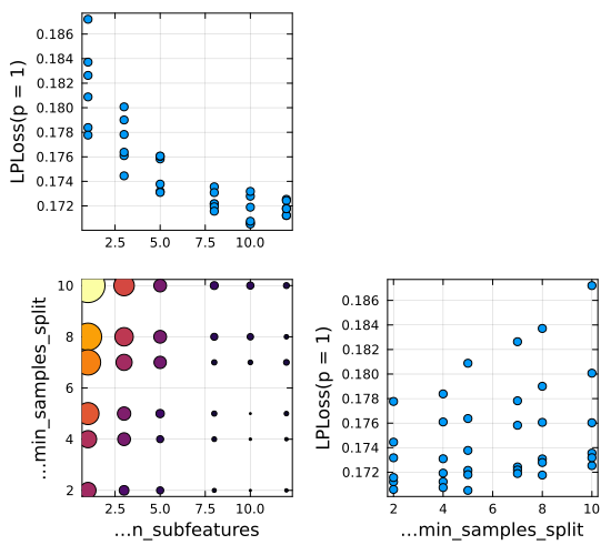
keys(report(mach))

(:best_model, :best_history_entry, :history, :best_report, :plotting)

report(mach).best_model

DeterministicPipeline(
  continuous_encoder = ContinuousEncoder(
        drop_last = false, 
        one_hot_ordered_factors = false), 
  random_forest_regressor = RandomForestRegressor(
        max_depth = -1, 
        min_samples_leaf = 1, 
        min_samples_split = 5, 
        min_purity_increase = 0.0, 
        n_subfeatures = 10, 
        n_trees = 250, 
        sampling_fraction = 0.7, 
        feature_importance = :impurity, 
        rng = 123), 
  cache = true)

report(mach).best_history_entry.evaluation

CompactPerformanceEvaluation object with these fields:
  model, measure, operation,
  measurement, per_fold, per_observation,
  resampling, repeats
Tag: 
Extract:
┌──────────┬───────────┬─────────────┐
│ measure  │ operation │ measurement │
├──────────┼───────────┼─────────────┤
│ LPLoss(  │ predict   │ 0.171       │
│   p = 1) │           │             │
└──────────┴───────────┴─────────────┘
┌─────────────────────────────┬─────────┐
│ per_fold                    │ 1.96*SE │
├─────────────────────────────┼─────────┤
│ [0.174, 0.16, 0.156, 0.192] │ 0.0181  │
└─────────────────────────────┴─────────┘

Instead we can use a random search strategy:

tuned_pipe = TunedModel(
    pipe,
    range=[r1, r2],
    tuning=RandomSearch(rng=123),
    resampling=CV(nfolds=4),
    measures=mae,
    n=40,
)

mach = machine(tuned_pipe, X, y) |> fit!
plt = plot(mach)

savefig("tuned_model_random.svg");

[ Info: Training machine(DeterministicTunedModel(model = DeterministicPipeline(continuous_encoder = ContinuousEncoder(drop_last = false, …), …), …), …).
[ Info: Attempting to evaluate 40 models.
Evaluating over 40 metamodels:   0%[>                        ]  ETA: N/A[KEvaluating over 40 metamodels:   2%[>                        ]  ETA: 0:00:32[KEvaluating over 40 metamodels:   5%[=>                       ]  ETA: 0:00:47[KEvaluating over 40 metamodels:   8%[=>                       ]  ETA: 0:00:44[KEvaluating over 40 metamodels:  10%[==>                      ]  ETA: 0:00:46[KEvaluating over 40 metamodels:  12%[===>                     ]  ETA: 0:00:53[KEvaluating over 40 metamodels:  15%[===>                     ]  ETA: 0:00:49[KEvaluating over 40 metamodels:  18%[====>                    ]  ETA: 0:00:47[KEvaluating over 40 metamodels:  20%[=====>                   ]  ETA: 0:00:46[KEvaluating over 40 metamodels:  22%[=====>                   ]  ETA: 0:00:47[KEvaluating over 40 metamodels:  25%[======>                  ]  ETA: 0:00:46[KEvaluating over 40 metamodels:  28%[======>                  ]  ETA: 0:00:43[KEvaluating over 40 metamodels:  30%[=======>                 ]  ETA: 0:00:42[KEvaluating over 40 metamodels:  32%[========>                ]  ETA: 0:00:40[KEvaluating over 40 metamodels:  35%[========>                ]  ETA: 0:00:40[KEvaluating over 40 metamodels:  38%[=========>               ]  ETA: 0:00:39[KEvaluating over 40 metamodels:  40%[==========>              ]  ETA: 0:00:37[KEvaluating over 40 metamodels:  42%[==========>              ]  ETA: 0:00:36[KEvaluating over 40 metamodels:  45%[===========>             ]  ETA: 0:00:34[KEvaluating over 40 metamodels:  48%[===========>             ]  ETA: 0:00:33[KEvaluating over 40 metamodels:  50%[============>            ]  ETA: 0:00:32[KEvaluating over 40 metamodels:  52%[=============>           ]  ETA: 0:00:30[KEvaluating over 40 metamodels:  55%[=============>           ]  ETA: 0:00:28[KEvaluating over 40 metamodels:  58%[==============>          ]  ETA: 0:00:27[KEvaluating over 40 metamodels:  60%[===============>         ]  ETA: 0:00:25[KEvaluating over 40 metamodels:  62%[===============>         ]  ETA: 0:00:24[KEvaluating over 40 metamodels:  65%[================>        ]  ETA: 0:00:22[KEvaluating over 40 metamodels:  68%[================>        ]  ETA: 0:00:21[KEvaluating over 40 metamodels:  70%[=================>       ]  ETA: 0:00:19[KEvaluating over 40 metamodels:  72%[==================>      ]  ETA: 0:00:17[KEvaluating over 40 metamodels:  75%[==================>      ]  ETA: 0:00:15[KEvaluating over 40 metamodels:  78%[===================>     ]  ETA: 0:00:14[KEvaluating over 40 metamodels:  80%[====================>    ]  ETA: 0:00:12[KEvaluating over 40 metamodels:  82%[====================>    ]  ETA: 0:00:11[KEvaluating over 40 metamodels:  85%[=====================>   ]  ETA: 0:00:09[KEvaluating over 40 metamodels:  88%[=====================>   ]  ETA: 0:00:08[KEvaluating over 40 metamodels:  90%[======================>  ]  ETA: 0:00:06[KEvaluating over 40 metamodels:  92%[=======================> ]  ETA: 0:00:05[KEvaluating over 40 metamodels:  95%[=======================> ]  ETA: 0:00:03[KEvaluating over 40 metamodels:  98%[========================>]  ETA: 0:00:02[KEvaluating over 40 metamodels: 100%[=========================] Time: 0:01:01[K

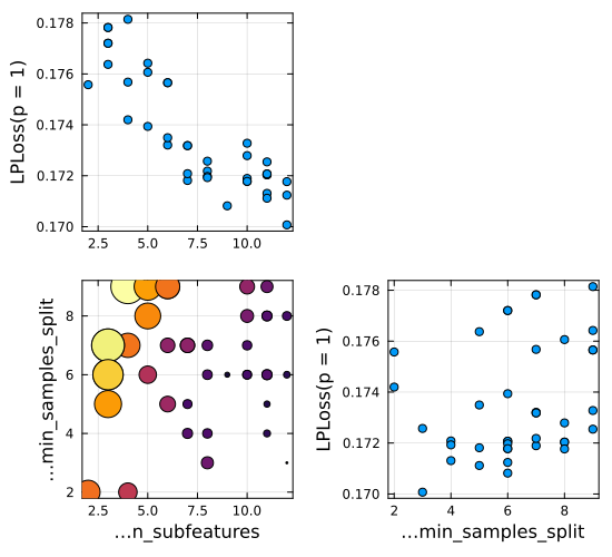
In-sample predictions based on optimized parameters and retraining on all data:

predict(mach, X)[1:5]

5-element Vector{Float64}:
 1.3710151999999998
 3.627463819999999
 1.8085951933333335
 1.9762690599999997
 1.3529714200000003

Evaluate the "self-tuning" pipeline:

e1 = evaluate(tuned_pipe, X, y; options...)

PerformanceEvaluation object with these fields:
  model, tag, measure, operation,
  measurement, uncertainty_radius_95, per_fold, per_observation,
  fitted_params_per_fold, report_per_fold,
  train_test_rows, resampling, repeats
Tag: DeterministicTunedModel-250
Extract:
┌──────────┬───────────┬─────────────┐
│ measure  │ operation │ measurement │
├──────────┼───────────┼─────────────┤
│ LPLoss(  │ predict   │ 0.175       │
│   p = 1) │           │             │
└──────────┴───────────┴─────────────┘
┌───────────────────────┬─────────┐
│ per_fold              │ 1.96*SE │
├───────────────────────┼─────────┤
│ [0.166, 0.166, 0.192] │ 0.021   │
└───────────────────────┴─────────┘

Comparing with the baseline computed earlier:

@show ebase e0 e1;

ebase = PerformanceEvaluation("ProbabilisticPipeline-112", 0.568 ± 0.0332)
e0 = PerformanceEvaluation("DeterministicPipeline-658", 0.184 ± 0.0281)
e1 = PerformanceEvaluation("DeterministicTunedModel-250", 0.175 ± 0.021)

Or, we can do this:

describe.([e0, e1]) |> pretty

┌─────────────────────────────┬──────────────────────┐
│ tag                         │ LPLoss               │
│ String                      │ Measurement{Float64} │
│ Textual                     │ Continuous           │
├─────────────────────────────┼──────────────────────┤
│ DeterministicPipeline-658   │ 0.184±0.028          │
│ DeterministicTunedModel-250 │ 0.175±0.021          │
└─────────────────────────────┴──────────────────────┘

We can also use TunedModel to compare models of different types:

tuned_model = TunedModel(models=[pipe, baseline], resampling=CV(nfolds=4), measure=l1)
mach = machine(tuned_model, X, y) |> fit!
report(mach).best_model

DeterministicPipeline(
  continuous_encoder = ContinuousEncoder(
        drop_last = false, 
        one_hot_ordered_factors = false), 
  random_forest_regressor = RandomForestRegressor(
        max_depth = -1, 
        min_samples_leaf = 1, 
        min_samples_split = 2, 
        min_purity_increase = 0.0, 
        n_subfeatures = 1, 
        n_trees = 250, 
        sampling_fraction = 0.7, 
        feature_importance = :impurity, 
        rng = 123), 
  cache = true)

Here tuned_model will behave just like pipe, because this is the best performer.

This page was generated using Literate.jl.

Lesson 3. Model Tuning

Part I. Learning Curves

Part II. The TunedModel Wrapper

Part II. The `TunedModel` Wrapper